User Guide
Introduction
To build and use and anomaly detection model with Amazon Lookout for Equipment, you need to go through the following steps:
Preparing your time series dataset and your historical maintenance time ranges
Upload your data on Amazon S3
Create a dataset and ingest the S3 data into it
Train a Lookout for Equipment model
Download and post-process the evaluation results
Configure and start a scheduler
Upload fresh data to Amazon S3
Download the inference results generated by the scheduler
The Amazon Lookout for Equipment SDK will help you streamline steps 3 to 8. Some sample datasets are also provided along with some utility functions to tackle steps 1 and 2.
Dataset management
Creating a dataset
Let’s start by loading a sample dataset and uploading it to a location on S3:
from lookoutequipment import dataset

root_dir = 'expander-data
bucket = '<<YOUR-BUCKET>>'     # Replace by your bucket name
prefix = '<<YOUR-PREFIX>>/'    # Don't forget the training slash
role_arn = '<<YOUR-ROLE-ARN>>' # An ARN role with access to your S3 data

data = dataset.load_dataset(
    dataset_name='expander',
    target_dir=root_dir
)
dataset.upload_dataset(root_dir, bucket, prefix)
From there we are going to instantiate a class that will help us manage our Lookout for Equipment dataset:
lookout_dataset = dataset.LookoutEquipmentDataset(
    dataset_name='my_dataset',
    access_role_arn=role_arn,
    component_root_dir=f'{bucket}/{prefix}training-data'
)
You will need to specify an ARN for a role that have access to your data on S3.
The following line creates the dataset in the Lookout for Equipment service. If you log into your AWS Console and browse to the Lookout for Equipment datasets list you will see an empty dataset:
lookout_dataset.create()
Ingesting data into a dataset
This dataset is empty: let’s ingest our prepared data (note the trailing slash at the end of the prefix):
response = lookout_dataset.ingest_data(bucket, prefix + 'training-data/')
The ingestion process will take a few minutes. If you would like to get a feedback from the ingestion process, you can enable a waiter by replacing the previous command by the following:
response = lookout_dataset.ingest_data(
    bucket,
    prefix + 'training-data/',
    wait=True,
    sleep_time=60
)
Model training
Once you have ingested some time series data in your dataset, you can train an anomaly detection model:
from lookoutequipment import model

lookout_model = model.LookoutEquipmentModel(model_name='my_model', dataset_name='my_dataset')
lookout_model.set_time_periods(data['evaluation_start'],
                               data['evaluation_end'],
                               data['training_start'],
                               data['training_end'])
lookout_model.set_label_data(bucket=bucket,
                             prefix=prefix + 'label-data/',
                             access_role_arn=role_arn)
lookout_model.set_target_sampling_rate(sampling_rate='PT5M')
response = lookout_model.train()
lookout_model.poll_model_training(sleep_time=300)
You will see a progress status update every five minutes until the training is successful. With the sample dataset used in this user guide, the training can take up to an hour.
Once your model is trained, you can either check the results over the evaluation period or configure an inference scheduler.
Evaluating a trained model
Plot detected events
Once a model is trained, the DescribeModel API from Amazon Lookout for Equipment will record the metrics associated to the training.
This API returns a dictionnary with two fields of interest to plot the
evaluation results: labelled_ranges and predicted_ranges which
respectively contain the known and predicted anomalies in the evaluation range.
Use the following SDK command to get both of these in a Pandas dataframe:
from lookoutequipment import evaluation

LookoutDiagnostics = evaluation.LookoutEquipmentAnalysis(model_name='my_model', tags_df=data['data'])
predicted_ranges = LookoutDiagnostics.get_predictions()
labeled_range = LookoutDiagnostics.get_labels()
Note: the labeled range from the DescribeModel API, only provides any labelled data falling within the evaluation range. If you want to plot or use all of them (including the labels falling within the training range), you should use the original label data by replacing the last line of the previous code snippet by the following code:
labels_fname = os.path.join(root_dir, 'labels.csv')
labeled_range = LookoutDiagnostics.get_labels(labels_fname)
You can then plot one of the original time series signal and add an overlay of the labeled and predicted anomalous events by levering the plot utilities:
from lookoutequipment import plot

TSViz = plot.TimeSeriesVisualization(timeseries_df=data['data'], data_format='tabular')
TSViz.add_signal(['signal-001'])
TSViz.add_labels(labeled_range)
TSViz.add_predictions([predicted_ranges])
TSViz.add_train_test_split(data['evaluation_start'])
TSViz.add_rolling_average(60*24)
TSViz.legend_format = {'loc': 'upper left', 'framealpha': 0.4, 'ncol': 3}
fig, axis = TSViz.plot()
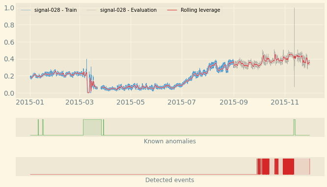
This code will generate the following plot where you can see:
A line plot for the signal selected: the part used for training the model appears in blue while the evaluation part is in gray.
The rolling average appears as a thin red line overlayed over the time series.
The labels are shown in a green ribbon labelled “Known anomalies” (by default)
The predicted events are shown in a red ribbon labelled “Detected events”
Plot signal distribution
You might be curious about why Amazon Lookout for Equipment detected an anomalous event. Sometime, looking at a few of the time series is enough. But sometime, you need to dig deeper.
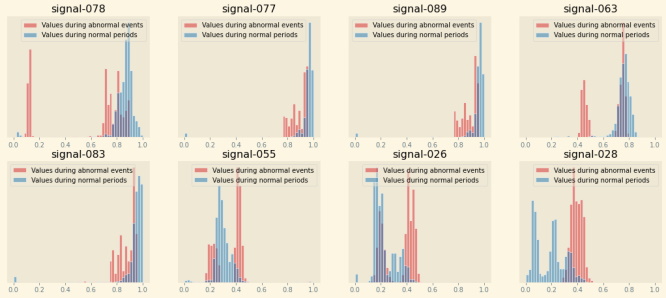
The following function, aggregate the signal importance of every signals over the evaluation period and sum these contributions over time for each signal. Then, it takes the top 8 signals and plot two distributions: one with the values each signal takes during the normal periods (present in the evaluation range) and a second one with the values taken during all the anomalous events detected in the evaluation range. This will help you visualize any significant shift of values for the top contributing signals.
You can also restrict these histograms over a specific range of time by setting
the start and end arguments of the following function with datetime
values:
from lookoutequipment import plot

TSViz = plot.TimeSeriesVisualization(timeseries_df=data['data'], data_format='tabular')
TSViz.add_predictions([predicted_ranges])
fig = TSViz.plot_histograms(freq='5min')
This code will generate the following plot where you can see a histogram for the top 8 signals contributing to the detected events present in the evaluation range of the model:
Scheduler management
Once a model is successfully trained, you can configure a scheduler that will run regular inferences based on this model:
from lookout import scheduler

lookout_scheduler = scheduler.LookoutEquipmentScheduler(
    scheduler_name='my_scheduler',
    model_name='my_model'
)

scheduler_params = {
    'input_bucket': bucket,
    'input_prefix': prefix + 'inference-data/input/',
    'output_bucket': bucket,
    'output_prefix': prefix + 'inference-data/output/',
    'role_arn': role_arn,
    'upload_frequency': 'PT5M',
    'delay_offset': None,
    'timezone_offset': '+00:00',
    'component_delimiter': '_',
    'timestamp_format': 'yyyyMMddHHmmss'
}

lookout_scheduler.set_parameters(**scheduler_params)
When the scheduler wakes up, it looks for the appropriate files in the input location configured above. It also opens each file and only keep the data based on their timestamp. Use the following command to prepare some inference data using the sample we have been using throughout this user guide:
dataset.prepare_inference_data(
    root_dir='expander-data',
    sample_data_dict=data,
    bucket=bucket,
    prefix=prefix
)
response = lookout_scheduler.create()
This will create a scheduler that will process one file every 5 minutes (matchin the upload frequency set when configuring the scheduler). After 15 minutes or so, you shoud have some results available. To get these results from the scheduler in a Pandas dataframe, you just have to run the following command:
results_df = lookout_scheduler.get_predictions()
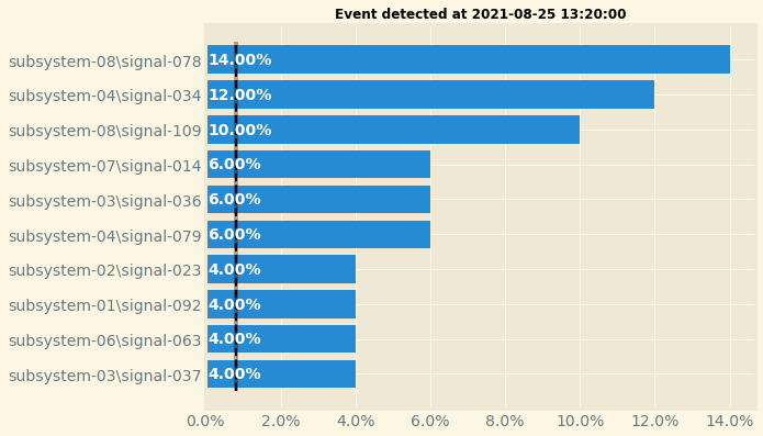
In this dataframe, you will find one row per event (i.e. one row per scheduler execution). You can then plot the feature importance of any given event. For instance, the following code will plot the feature importance for the first inference execution result:
event_details = pd.DataFrame(results_df.iloc[0, 1:]).reset_index()
fig, ax = plot.plot_event_barh(event_details)
This is the result you should have with the sample data:
Once you’re done, do not forget to stop the scheduler to stop incurring cost:
scheduler.stop()
You can restart your scheduler with a call to scheduler.start() and when
you don’t have any more use for your scheduler you can delete a stopped scheduler
by running scheduler.delete().